Multivariate Linear Regression

Multiple Features

Linear regression with multiple variables is also known as “multivariate linear regression”. We now introduce notation for equations where we can have any number of input variables.

$\begin{align*}x_j^{(i)} &= \text{value of feature } j \text{ in the }i^{th}\text{ training example} \newline x^{(i)}& = \text{the input (features) of the }i^{th}\text{ training example} \newline m &= \text{the number of training examples} \newline n &= \text{the number of features} \end{align*}$

The multivariable form of the hypothesis function accommodating these multiple features is as follows:

$h_θ(x)=θ_0+θ_1x_1+θ_2x_2+θ_3x_3+⋯+θ_nx_n$

In order to develop intuition about this function, we can think about $\theta_0$ as the basic price of a house, $\theta_1$ as the price per square meter, $\theta_2$ as the price per floor, etc. $x_1$ will be the number of square meters in the house, $x_2$ the number of floors, etc.

Using the definition of matrix multiplication, our multivariable hypothesis function can be concisely represented as:

$\begin{align*}h_\theta(x) =\begin{bmatrix}\theta_0 \hspace{2em} \theta_1 \hspace{2em} ... \hspace{2em} \theta_n\end{bmatrix}\begin{bmatrix}x_0 \newline x_1 \newline \vdots \newline x_n\end{bmatrix}= \theta^T x\end{align*}$

This is a vectorization of our hypothesis function for one training example; see the lessons on vectorization to learn more.

Remark: Note that for convenience reasons in this course we assume $x^{(i)}_0=1 $ for $(i\in 1,\dots,m)$. This allows us to do matrix operations with theta and x. Hence making the two vectors $’\thetaθ’$ and $x^{(i)}$match each other element-wise (that is, have the same number of elements: n+1).]

Gradient Descent for Multiple Variables

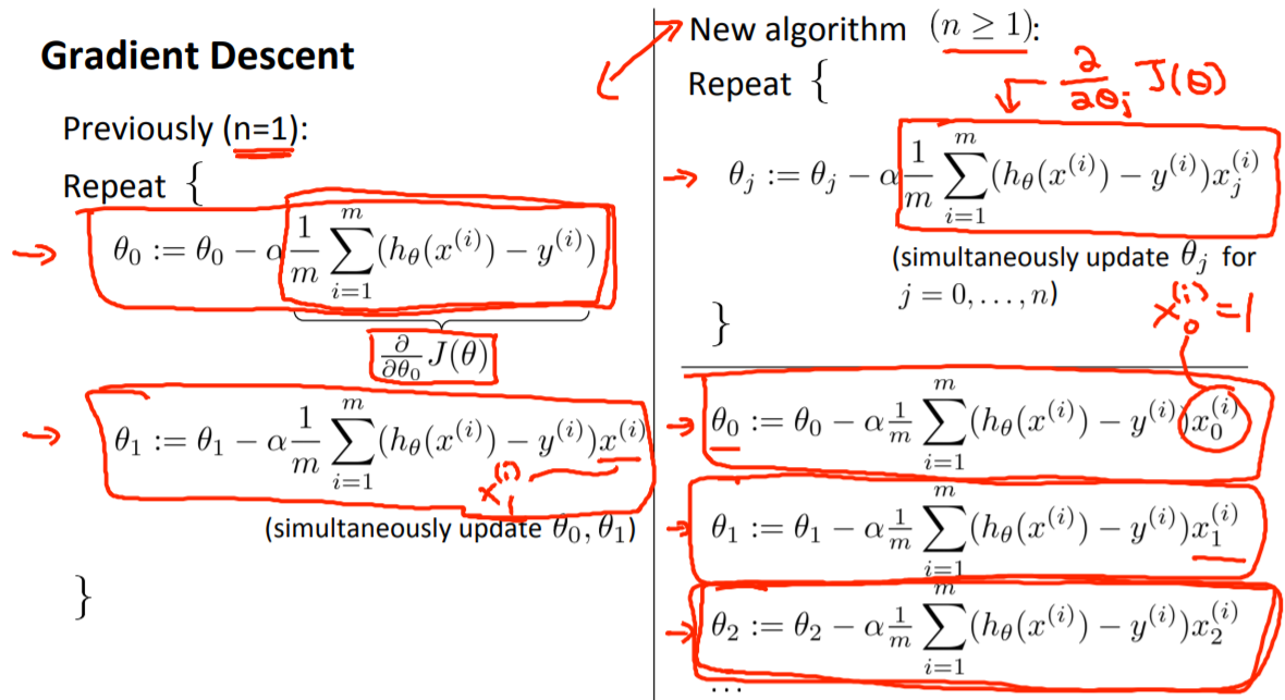
The gradient descent equation itself is generally the same form; we just have to repeat it for our ‘n’ features:

$\begin{align} & \text{repeat until convergence:} \; \lbrace \newline \; & \theta_0 := \theta_0 - \alpha \frac{1}{m} \sum\limits_{i=1}^{m} (h_\theta(x^{(i)}) - y^{(i)}) \cdot x_0^{(i)}\newline \; & \theta_1 := \theta_1 - \alpha \frac{1}{m} \sum\limits_{i=1}^{m} (h_\theta(x^{(i)}) - y^{(i)}) \cdot x_1^{(i)} \newline \; & \theta_2 := \theta_2 - \alpha \frac{1}{m} \sum\limits_{i=1}^{m} (h_\theta(x^{(i)}) - y^{(i)}) \cdot x_2^{(i)} \newline & \cdots \newline \rbrace \end{align}$

In other words:

$\begin{align*}& \text{repeat until convergence:} \; \lbrace \newline \; & \theta_j := \theta_j - \alpha \frac{1}{m} \sum\limits_{i=1}^{m} (h_\theta(x^{(i)}) - y^{(i)}) \cdot x_j^{(i)} \; & \text{for j := 0...n}\newline \rbrace\end{align*}$

The following image compares gradient descent with one variable to gradient descent with multiple variables:

Python代码示例：

计算代价函数：$J\left( \theta \right)=\frac{1}{2m}\sum\limits_{i=1}^{m}{\left( h_{\theta}\left( x^{(i)} \right)-y^{(i)} \right)}^2$
其中：$h_{\theta}\left( x \right)=\theta^{T}X=\theta_{0}x_{0}+\theta_{1}x_{1}+\theta_{2}x_{2}+…+\theta_{n}x_{n}$

1
2
3

def computeCost(X, y, theta):
    inner = np.power(((X * theta.T) - y), 2)
    return np.sum(inner) / (2 * len(X))

Gradient Descent in Practice I -Feature Scaling

We can speed up gradient descent by having each of our input values in roughly the same range. This is because θ will descend quickly on small ranges and slowly on large ranges, and so will oscillate inefficiently down to the optimum when the variables are very uneven.

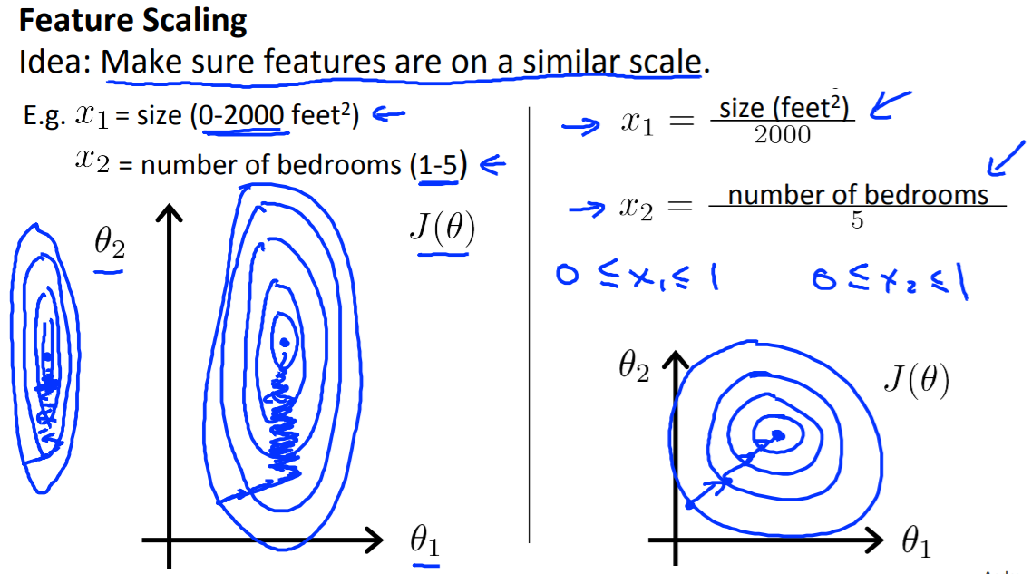
The way to prevent this is to modify the ranges of our input variables so that they are all roughly the same. Ideally:

−1 ≤ $x_{(i)}$≤ 1 or −0.5 ≤ $x_{(i)}$ ≤ 0.5

Two techniques to help with this are feature scaling(特征缩放) and mean normalization(均值归一化).

Feature scaling involves dividing the input values by the range (maximum value - minimum value) of the input variable, resulting in a new range of just 1.

Mean normalization involves subtracting the average value for an input variable from the values for that input variable resulting in a new average value for the input variable of just zero. To implement both of these techniques, adjust your input values as shown in this formula:

$x_i:=\frac{x_i-\mu_i}{s_i}$

Where $\mu_i$ is the average of all the values for feature (i) and $s_i$ is the range of values (max - min), or $s_i$ is the standard deviation(标准差). （量化后的特征将分布在[-1, 1]，服从标准正态分布）

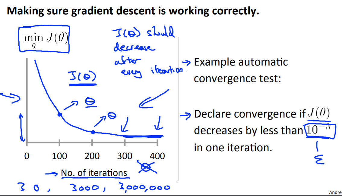
Gradient Descent in Practice II - Learning Rate

Debugging gradient descent(调试梯度下降): Make a plot with number of iterations on the x-axis. Now plot the cost function, J(θ) over the number of iterations of gradient descent. If J(θ) ever increases, then you probably need to decrease α.

Automatic convergence test(自动收敛测试): Declare convergence if J(θ) decreases by less than E in one iteration, where E is some small value such as 10−3. However in practice it’s difficult to choose this threshold value

It has been proven that if learning rate α is sufficiently small, then J(θ) will decrease on every iteration.

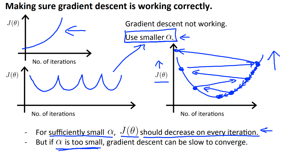
To summarize:

If $\alpha$ is too small: slow convergence.
If $\alpha$ is too large: may not decrease on every iteration and thus may not converge.

Features and Polynomial Regression

We can improve our features and the form of our hypothesis function in a couple different ways.

We can combine multiple features into one. For example, we can combine $x_1$ and $x_2$ into a new feature $x_3$ by taking $x_1⋅x_2$.

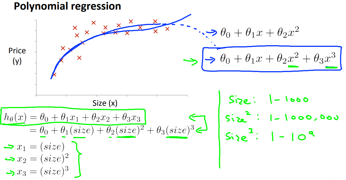
Our hypothesis function need not be linear (a straight line) if that does not fit the data well.

We can change the behavior or curve of our hypothesis function by making it a quadratic, cubic or square root function (or any other form).

For example, if our hypothesis function is $h_\theta (x) = \theta_0 + \theta_1 x_1$ then we can create additional features based on $x_1$, to get the quadratic function $h_\theta(x) = \theta_0 + \theta_1 x_1 + \theta_2 x_1^2$ or the cubic function $h_\theta(x) = \theta_0 + \theta_1 x_1 + \theta_2 x_1^2 + \theta_3 x_1^3$

In the cubic version, we have created new features $x_2$ and $x_3$ where $x_2 = x_1^2$ and $x_3 = x_1^3$.

To make it a square root function, we could do: $h_\theta(x) = \theta_0 + \theta_1 x_1 + \theta_2 \sqrt{x_1}$.

One important thing to keep in mind is, if you choose your features this way then feature scaling becomes very important.

eg. if $x_1$ has range 1 - 1000 then range of $x_1^2$ becomes 1 - 1000000 and that of $x_1^3$ becomes 1 - 1000000000

Normal Equation

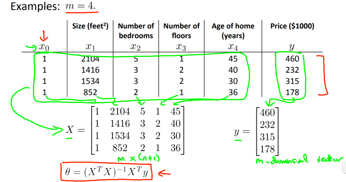
Gradient descent gives one way of minimizing J. Let’s discuss a second way of doing so, this time performing the minimization explicitly and without resorting to an iterative algorithm. In the “Normal Equation“ (正规方程) method, we will minimize J by explicitly taking its derivatives with respect to the θj ’s, and setting them to zero: $\frac{\partial J\left( \theta \right)}{\partial \theta }=0$.

This allows us to find the optimum theta without iteration. The normal equation formula is given below:

$\theta = (X^T X)^{-1}X^T y$

There is no need to do feature scaling with the normal equation.

The following is a comparison of gradient descent and the normal equation:

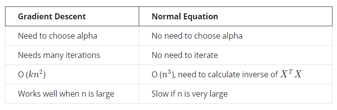
总结一下，只要特征变量的数目并不大，标准方程是一个很好的计算参数$\theta $的替代方法。具体地说，只要特征变量数量小于一万，我通常使用标准方程法，而不使用梯度下降法。

随着学习算法越来越复杂，例如，分类算法，像逻辑回归算法，我们会看到，实际上对于那些算法，并不能使用标准方程法。对于那些更复杂的学习算法，我们将不得不仍然使用梯度下降法。因此，梯度下降法是一个非常有用的算法，可以用在有大量特征变量的线性回归问题。但对于这个特定的线性回归模型，标准方程法是一个比梯度下降法更快的替代算法。所以，根据具体的问题，以及特征变量的数量，这两种算法都是值得学习的。

正规方程的python实现：

import numpy as np
    
 def normalEqn(X, y):
    
   theta = np.linalg.inv(X.T@X)@X.T@y #X.T@X等价于X.T.dot(X)
    
   return theta

Noninvertibility(不可逆性)

When implementing the normal equation in octave we want to use the pinv function rather than inv. The ‘pinv‘ function will give you a value of $\theta$ even if $X^TX$ is not invertible.

If $X^TX$ is noninvertible, the common causes might be having :

Redundant features, where two features are very closely related (i.e. they are linearly dependent)
Too many features (e.g. m ≤ n). In this case, delete some features or use “regularization“（正则化） (to be explained in a later lesson).

Solutions to the above problems include deleting a feature that is linearly dependent with another or deleting one or more features when there are too many features.

补充：$\theta = (X^T X)^{-1}X^T y$的证明：

代价函数：

$J\left( \theta \right)=\frac{1}{2m}\sum\limits_{i=1}^{m}{\left( h_{\theta}\left( x^{(i)} \right)-y^{(i)} \right)}^2$

其中：$h_{\theta}\left( x \right)=\theta^{T}X=\theta_{0}x_{0}+\theta_{1}x_{1}+\theta_{2}x_{2}+…+\theta_{n}x_{n}$

将向量表达形式转为矩阵表达形式，则有$J(\theta )=\frac{1}{2}{\left( X\theta -y\right)}^2$ ，其中$X$为$m$行$n$列的矩阵（$m$为样本个数，$n$为特征个数），$\theta$为$n$行1列的矩阵，$y$为$m$行1列的矩阵，对$J(\theta )$进行如下变换

$\begin{align}J(\theta )&=\frac{1}{2}{\left( X\theta -y\right)}^{T}\left( X\theta -y \right) \\ &=\frac{1}{2}\left( {\theta }^{T}{X^T}-{y}^{T} \right)\left(X\theta -y \right)\\&=\frac{1}{2}\left( {\theta }^T{X}^{T}X\theta -{\theta}^{T}{X}^{T}y-{y}^{T}X\theta -{y}^{T}y \right) \end{align}$

接下来对$J(\theta )$偏导，需要用到以下几个矩阵的求导法则

$\begin{align} \frac{dAB}{dB}&={A^T}\\\frac{dX^TAX}{dX}&=2AX \end{align}$

所以有:

$\begin{align} \frac{\partial J\left( \theta \right)}{\partial \theta }&=\frac{1}{2}\left(2{X^T}X\theta -{X^T}y -({y^T}X )^{T}-0 \right)\\&=\frac{1}{2}\left(2{X^T}X\theta -{X^T}y -{X^T}y -0 \right)\\&={X^T}X\theta -{X^T}y \end{align}$

令：$\frac{\partial J\left( \theta \right)}{\partial \theta }=0$

则有：$\theta =\left( X^{T}X \right)^{-1}{X^T}y$。

————————————————————————————————————————————————

PS：Week2的第三部分是Octave语言教程，看了一遍视频发现Octave的语法和Matlab基本是一样的，有很方便的矩阵运算，而且Octave是完全开源的，但正版的Matlab确实很贵，这大概也是老师这门课用Octave的原因之一吧。（Andrew Ng 永远滴神！）